SPPU Previous Year UNIT-I Question and Answer of ML asked in Insem Examination

 Show how machine learning differs from traditional programming.  Elaborate with suitable diagram.

Machine learning vs. traditional programming

 

 

 

 

While both traditional programming and machine learning aim to solve problems using computers, they fundamentally differ in their approach to how the computer arrives at a solution. 

Traditional programming

In traditional programming, a programmer explicitly defines a set of rules, instructions, or algorithms that the computer follows to process input data and produce a desired output. The logic and steps are meticulously crafted by humans, and the system executes them deterministically. 

Traditional programming model diagram

Input -> Explicit Instructions (Program) -> Output

Machine learning

In contrast, machine learning involves training a model using a large dataset. Instead of being given explicit instructions for every possible scenario, the machine learning model learns patterns and relationships from the data and uses this learned knowledge to make predictions or decisions on new, unseen data. The model adapts and improves over time with more data and experience. 

Machine learning model diagram

Input + Output (Data) -> Machine Learning Algorithm -> Learned Model

 

New Input -> Learned Model -> Predicted Output

Both Machine Learning programming and traditional programming serve businesses in different ways.

• Traditional programming follows fixed rules, making it ideal for predictable tasks.
• Machine Learning programming allows systems to learn from data and improve over time.

Here’s a more detailed comparison between the programming of Machine Learning and traditional programming:

Factors	Traditional Programming	Machine Learning programming
Instruction method	Explicit rules and logic	Learns patterns from data
Handling data	Processes structured data	Works with large, unstructured data
Outcome predictability	Always produces the same result	Predictions vary based on training
Decision making	Rule-based	Machine Learning decision making
Flexibility	Limited to predefined conditions	Adjusts based on new data

Traditional programming requires structured inputs, meaning data must be formatted consistently.

Data quality for Machine Learning is critical because ML systems learn from past examples, making them dependent on accurate and diverse datasets.

1. Flexibility & adaptability

Traditional software operates within set boundaries.

Machine Learning adapts over time, making it useful for dynamic environments like fraud detection or Machine Learning for business decisions.

2. Problem complexity

Rule-based systems handle straightforward tasks well, but they struggle with complex problems like image recognition or language processing.

Hybrid Machine Learning models are often used to tackle multi-layered challenges, offering more sophisticated solutions.

3. Decision-making & predictability

Traditional programming provides clear, consistent outputs.

Machine Learning, in contrast, offers probability-based predictions, making it valuable for scenarios where patterns evolve over time, such as Machine Learning business applications.

4. Transparency & explainability

Traditional programming follows clear rules, making decisions easy to trace.

Explainable AI helps businesses interpret ML predictions, ensuring reliability in sensitive applications like finance and healthcare.

Key differences

The core distinctions between the two can be summarized as follows:

• Instruction method: Traditional programming relies on explicitly coded rules and logic. Machine learning, on the other hand, learns patterns from data.
• Handling data: Traditional programming is best suited for structured, well-defined problems where data inputs are consistent. Machine learning thrives on large, complex, and often unstructured datasets where patterns are not easily discernible through explicit rules.
• Outcome predictability: Traditional programming yields predictable and consistent results when given the same inputs. Machine learning outputs can vary due to the probabilistic nature of its predictions and its ability to adapt to new information.
• Adaptability: Traditional programs require manual updates for new scenarios or changes in requirements. Machine learning models, conversely, adjust and improve based on new data, reducing the need for constant manual intervention.
• Problem complexity: Traditional programming excels at tasks with clear, deterministic logic. Machine learning is better equipped for complex problems like image recognition, natural language processing, or fraud detection where patterns are intricate and not easily encoded into fixed rules. 

Example: fraud detection

Imagine a system to detect fraudulent transactions:

• Traditional Programming Approach: A programmer would define a set of explicit rules: "If a transaction amount exceeds X AND is from country Y AND the account has been active for less than Z days, flag as potentially fraudulent". This approach is effective if all fraudulent scenarios can be anticipated and explicitly coded.
• Machine Learning Approach: Instead of predefined rules, a machine learning model would be trained on historical transaction data, including information about past fraudulent and legitimate transactions. The model learns to identify complex patterns and relationships that distinguish fraudulent activity from normal behavior, without being explicitly programmed for every possible fraud signature. This allows it to adapt to new and evolving fraud schemes more effectively. 

 

Both traditional programming and machine learning are powerful tools, each suited for different problem types. Traditional programming provides precise control and predictable outcomes for rule-based systems. Machine learning excels in complex environments, where it can learn from data, adapt to changes, and uncover insights that might be missed by explicit rule-based systems. Often, a combination of both approaches, known as hybrid models, can be employed to leverage the strengths of both for building robust and intelligent systems. 

 

 Explain K-fold Cross Validation technique with suitable example.

 

The concept of cross-validation is widely used in data science and machine learning. It’s a way to verify the performance of a predictive model before using it in an actual situation. Essentially, it helps you avoid creating inaccurate predictions. Using multiple training sets is crucial when performing cross-validation. You must have multiple test sets to ensure your model performs as expected. In this article we are going to learn about K-fold Cross-validation.

In K-fold cross-validation, the data set is divided into a number of K-folds and used to assess the model’s ability as new data become available. K represents the number of groups into which the data sample is divided. For example, if you find the k value to be 5, you can call it 5-fold cross-validation. Each fold is used as a test set at some point in the process.

·         Randomly shuffle the dataset.

·         Divide the dataset into k folds

·         For each unique group:

·         Use one fold as test data

·         Use remaining groups as training dataset

·         Fit model on training set and evaluate on test set

·         Keep Score 

4. Get accuracy score by applying mean to all the accuracies received for all folds.

As you can see in the fig that there is a dataset which is Divided into 5 folds. That means there will be five iterations, and in each iteration, there will be one test fold, and the other four folds will be training folds. And in each iteration, test and training folds keep on changing. That means if we have 1000 records in our data set, then suppose 200 records are our test data, and 800 records are our training data. 

So in the first iteration, (1-200) records will be test data, and (201-1000) will be training data. In the second iteration, (1-200) records plus (401-1000) represent training data, And (200 -400) will represent the test data.

 

Advantages of K-fold cross validation

·         Stable accuracy: This will solve the random precision issue. In other words, stable accuracy can be achieved. The model is trained on a dataset split into multiple folds. 

·         Overfitting: This prevents the overfitting of the training data set.

·         Model Generalization Validation: Cross-validation gives insight into how the model generalizes to unknown data sets

·         Validate model performance: Cross-validation allows you to accurately estimate your model’s predictive performance.

 

 Disadvantages of K-fold cross validation

·         Don’t work on an imbalanced dataset: If your data is imbalanced (if you have class “A” and class “B,” the training set has class “A” and the test set has class “B”), it doesn’t work well.

·         Increased training time: Cross-validation requires training the model on multiple training sets.

·         Computationally expensive: Cross-validation is computationally expensive as it needs to be trained on multiple training sets.

 

 

 

What is Dataset? Differentiate between Training dataset and Testing dataset.

A data set (or dataset) is a collection of data. In the case of tabular data, a data set corresponds to one or more database tables, where every column of a table represents a particular variable, and each row corresponds to a given record of the data set in question.

OR

A dataset is a collection of data, often organized into rows and columns, that can be used for various purposes, including machine learning, research, and statistical analysis. Datasets can contain different types of information, such as numbers, text, images, or audio, and can be stored in various formats. 

Differentiating between training and testing datasets

In the development of a machine learning model, a dataset is typically split into training and testing subsets.

• Training dataset:
• This is the portion of the data used to train the machine learning model.
• It contains labeled examples (input features and corresponding target labels) that help the model learn patterns and relationships within the data.
• The model uses this data to adjust its internal parameters (weights) to minimize errors and improve its ability to make accurate predictions.
• Typically, the training set is a larger portion of the overall dataset, such as 70-80%.
• Testing dataset:
• This is a separate subset of data used to evaluate the performance of the trained model on unseen data.
• It also contains input features and corresponding target labels but is not used during the training phase.
• The purpose of the testing set is to provide an unbiased assessment of how well the model generalizes to new, real-world data and avoids overfitting.
• The testing set is typically a smaller portion of the overall dataset, such as 20-30%. 

 

Parameter	Training Data	Testing Data
Purpose	Used to train and teach the model.	Used to evaluate model performance.
Data Type	Labeled data with known outputs.	Unseen data to check generalization.
Role	Helps the model learn patterns and relationships.	Assesses accuracy and effectiveness.
Usage	Fed into the model for learning.	Used after training to test the model.
Quantity	Larger dataset to ensure better learning.	Smaller dataset compared to training data.
Effect on Model	Helps improve accuracy through multiple iterations.	Detects issues like overfitting and underfitting.
Evaluation Metrics	Not used for accuracy measurement.	Used to measure accuracy, precision, recall, etc.
Adjustments	Model parameters are adjusted during training.	No adjustments are made; only evaluation is done.
Risk	Overfitting if the model learns too much from training data.	Poor evaluation if the testing data is not diverse.
Final Output	Creates a trained model.	Validates the model before deployment.

 

Compare Supervised, Unsupervised and Semi-supervised Learning with examples.

Supervised Learning:

• Definition:

In supervised learning, the algorithm learns from a labeled dataset, where each data point has a corresponding correct output (label). 

• Goal:

The goal is to learn a mapping function that can predict the output for new, unseen data based on the labeled training data. 

• Examples:

• Spam detection: Classifying emails as spam or not spam based on labeled examples of both. 

• Image recognition: Identifying objects in images (e.g., cats vs. dogs) based on labeled training data. 

• Price prediction: Predicting the price of a house based on features like size, location, and number of bedrooms, using historical data with known prices. 

Unsupervised Learning:

• Definition:

Unsupervised learning algorithms work with unlabeled data, meaning there are no predefined correct outputs for the algorithm to learn from. 

• Goal:

The goal is to discover hidden structures, patterns, or relationships within the data. 

• Examples:

• Customer segmentation: Grouping customers based on their purchasing behavior to identify distinct customer segments. 

• Anomaly detection: Identifying unusual data points or patterns that deviate from the norm, such as fraudulent transactions or network intrusions. 

• Dimensionality reduction: Reducing the number of variables in a dataset while preserving important information. 

Semi-Supervised Learning:

• Definition:

Semi-supervised learning combines the strengths of both supervised and unsupervised learning by using both labeled and unlabeled data. 

• Goal:

To leverage a small amount of labeled data to guide the learning process on a larger amount of unlabeled data, improving model performance compared to using only labeled or unlabeled data alone. 

• Examples:

• Image classification with a small labeled set: Using a small set of images with labels (e.g., cat or dog) to train a model, then using the model to classify a much larger set of unlabeled images. 

• Sentiment analysis with a small set of labeled reviews: Classifying movie reviews as positive or negative, using a small set of labeled reviews to guide the classification of a much larger set of unlabeled reviews. 

 

Here's a comparison of Supervised, Unsupervised, and Semi-supervised Learning:

Aspect	Supervised Learning	Unsupervised Learning	Semi-supervised Learning
Data Used	Labeled data (input data with corresponding correct output labels)	Unlabeled data (input data without output labels)	Combination of a small amount of labeled data and a large amount of unlabeled data
Goal	Predict outcomes for new data based on patterns learned from labeled examples.	Discover hidden patterns, structures, or relationships within the data without predefined outcomes.	Improve model performance and accuracy, especially when labeled data is scarce but unlabeled data is abundant.
Algorithms	Regression (e.g., Linear Regression) and Classification (e.g., Decision Trees, Logistic Regression, Support Vector Machines).	Clustering (e.g., K-Means, Hierarchical Clustering) and Dimensionality Reduction (e.g., Principal Component Analysis).	Techniques that combine aspects of supervised and unsupervised learning, such as self-training or co-training.
Examples	Spam detection, Image classification, Sentiment analysis, Predicting house prices	Customer segmentation, Anomaly detection, Recommendation systems	Web page classification, Speech analysis, Protein sequence classification
Human Effort	High, required for labeling data.	Less, primarily for interpreting the discovered patterns.	Moderate, some labeling is required, but less than fully supervised learning.
Accuracy	Generally high, as it's guided by known correct answers.	Can be lower and vary depending on the data and algorithm.	Can achieve better accuracy than unsupervised methods when limited labeled data is available.
Adaptability	Less adaptable to changes in data distribution without retraining.	Can adapt to new data patterns, but may require re-tuning.	Moderately adaptable, as it can utilize unlabeled data to improve.
Complexity	Generally more straightforward.	Can be complex due to the lack of labels and need to interpret patterns.	Intermediate complexity, combining aspects of both supervised and unsupervised learning.

 

What is the need of dimensionality reduction? Explain subset selection method.

 

Dimensionality reduction simplifies data analysis, visualization, and model building by reducing the number of features while preserving essential information. Feature subset selection is a dimensionality reduction technique that involves choosing a relevant subset of the original features to improve model performance, reduce overfitting, and enhance interpretability. 

Need for Dimensionality Reduction:

• Simplifies data:

High-dimensional data can be difficult to analyze and visualize, making dimensionality reduction crucial for understanding patterns and relationships within the data. 

• Reduces computational cost:

Fewer features mean less computation, saving time and resources, especially for large datasets. 

• Prevents overfitting:

Irrelevant features can lead to overfitting, where a model performs well on training data but poorly on new, unseen data. Dimensionality reduction can mitigate this by removing noisy or redundant features. 

• Improves model interpretability:

Simpler models with fewer features are often easier to understand and interpret, leading to better insights. 

• Reduces storage space:

Fewer features require less storage space, which can be particularly beneficial for large datasets. 

Feature Subset Selection:

Feature subset selection is a dimensionality reduction technique that focuses on selecting a subset of the original features without transforming them. This contrasts with feature extraction, which creates new features from the original ones. 

Methods of Feature Subset Selection:

1. Filter Methods:

These methods evaluate the relevance of features based on their statistical properties, such as correlation with the target variable or variance. Examples include:

·         Correlation-based feature selection: Selects features with high correlation to the target variable.

·         Variance threshold: Removes features with low variance, as they may not contribute much to the model.

·         Information gain: Measures the amount of information a feature provides about the target variable.

2. Wrapper Methods:

These methods evaluate feature subsets by training a machine learning model with each subset and assessing its performance. Examples include:

·         Recursive Feature Elimination (RFE): Iteratively removes the least important features based on model performance.

·         Forward Selection: Starts with an empty set of features and iteratively adds the most relevant feature until a stopping criterion is met.

·         Backward Elimination: Starts with all features and iteratively removes the least relevant feature until a stopping criterion is met.

3. Embedded Methods:

These methods incorporate feature selection as part of the model training process. Examples include:

·         LASSO regularization: Adds a penalty term to the model's loss function that encourages sparsity, effectively selecting a subset of features.

·         Ridge Regression: Similar to LASSO, but uses a different penalty term that encourages all features to have small weights. 

 

 

What is feature? Explain types of feature selection technique.

 

In machine learning and data analysis, a feature is an individual, measurable property or characteristic of the data being observed. They are the input variables or attributes that a model uses to make predictions or classifications. For example, in a dataset used to predict house prices, features could include the number of bedrooms, square footage, and location. 

Types of Feature Selection Techniques:

1.     Filter Methods

2.     Wrapper Methods

3.     Embedded Methods

Each one has its own strengths and trade-offs depending on the use case.

1. Filter Methods

Filter methods evaluate each feature independently with target variable. Feature with high correlation with target variable are selected as it means this feature has some relation and can help us in making predictions. These methods are used in the preprocessing phase to remove irrelevant or redundant features based on statistical tests (correlation) or other criteria.

                                                                           Filter Methods Implementation

Advantages:

·         Quickly evaluate features without training the model.

·         Good for removing redundant or correlated features.

 

2. Wrapper methods

Wrapper methods are also referred as greedy algorithms that train algorithm. They use different combination of features and compute relation between these subset features and target variable and based on conclusion addition and removal of features are done. Stopping criteria for selecting the best subset are usually pre-defined by the person training the model such as when the performance of the model decreases or a specific number of features are achieved.

                                                      Wrapper Methods Implementation

Advantages:

·         Can lead to better model performance since they evaluate feature subsets in the context of the model.

·         They can capture feature dependencies and interactions.

Limitations: They are computationally more expensive than filter methods especially for large datasets.

Some techniques used are:

·         Forward selection: This method is an iterative approach where we initially start with an empty set of features and keep adding a feature which best improves our model after each iteration. The stopping criterion is till the addition of a new variable does not improve the performance of the model.

·         Backward elimination: This method is also an iterative approach where we initially start with all features and after each iteration, we remove the least significant feature. The stopping criterion is till no improvement in the performance of the model is observed after the feature is removed.

·         Recursive elimination: Recursive elimination is a greedy method that selects features by recursively removing the least important ones. It trains a model, ranks features based on importance and eliminates them one by one until the desired number of features is reached.

3. Embedded methods

Embedded methods perform feature selection during the model training process. They combine the benefits of both filter and wrapper methods. Feature selection is integrated into the model training allowing the model to select the most relevant features based on the training process dynamically.

                                              Embedded Methods Implementation

Advantages:

·         More efficient than wrapper methods because the feature selection process is embedded within model training.

·         Often more scalable than wrapper methods.

Limitations: Works with a specific learning algorithm so the feature selection might not work well with other models

Some techniques used are:

·         L1 Regularization (Lasso): A regression method that applies L1 regularization to encourage sparsity in the model. Features with non-zero coefficients are considered important.

·         Decision Trees and Random Forests: These algorithms naturally perform feature selection by selecting the most important features for splitting nodes based on criteria like Gini impurity or information gain.

·         Gradient Boosting: Like random forests gradient boosting models select important features while building trees by prioritizing features that reduce error the most.

 

 

Why dataset splitting is required? State importance of each split in a machine learning model.

 

In machine learning, dataset splitting is crucial for building and evaluating models that can generalize well to new, unseen data. The goal of machine learning is not just to perform well on the data it was trained on but to also make accurate predictions on data it has never encountered before. Data splitting helps achieve this by creating distinct sets of data for different stages of model development.

 Enhancing Model Performance: Data splitting enables candidates to validate and evaluate machine learning models effectively. By evaluating the model's performance on independent test sets, candidates can identify areas for improvement, fine-tune their models, and enhance overall predictive accuracy.

 

  Importance of each split:

·         Training Set:

This is the largest subset of data, used to train the machine learning model. The model learns patterns, relationships, and features from this data to build its internal representation. 

·         Validation Set:

This set is used to fine-tune the model's hyperparameters and architecture during the training process. It helps prevent overfitting, where the model performs well on the training data but poorly on new data. By evaluating the model's performance on the validation set, we can make adjustments to prevent the model from memorizing the training data. 

·         Testing Set:

This set is kept completely separate from the training and validation processes. It's used to assess the model's performance on unseen data, providing an unbiased evaluation of its generalization ability. The test set helps determine how well the model will perform in real-world scenarios. 

 

By splitting the dataset appropriately, we can ensure that the model is not only trained effectively but also generalizes well to new, unseen data, leading to more reliable and robust machine learning models. 

 

 

Why size of training dataset is more compare to testing dataset? What should be ratio of Training & testing dataset? Explain any one dataset validation techniques.

 

In machine learning, the training dataset is typically larger than the testing dataset to provide the model with sufficient data to effectively learn the underlying patterns and relationships. 

Here's why:

• Effective Learning: A larger training dataset allows the model to be exposed to a broader range of examples and variations, enabling it to learn the features and characteristics needed to make accurate predictions or perform the desired task.
• Generalization: With more training data, the model can better generalize its learning to new, unseen data, which is crucial for achieving good performance on real-world applications.
• Preventing Underfitting: If the training dataset is too small, the model might not capture enough patterns or relationships, leading to poor performance on new data (underfitting).
• Model Accuracy: The precision of a machine learning model is sensitive to the quantity of training data. In most cases, accuracy improves with a larger training dataset. 

Ratio of Training and Testing Dataset

While there is no universally fixed rule, common ratios for splitting data into training and testing sets are: 

• 70% Training / 30% Testing
• 80% Training / 20% Testing 

However, the optimal ratio depends on several factors, including: 

• Dataset Size: For large datasets (millions of records), even a smaller percentage like 1% for testing may be sufficient (e.g., 98% training / 1% validation / 1% testing).
• Model Complexity: Complex models or those with a high number of parameters benefit from larger training sets.
• Computational Resources: Larger training sets require more computational resources and time for model training. 

Dataset Validation Techniques

K-fold Cross-validation is a widely used dataset validation technique. 

Here's how it works:

1.     Divide into K Folds: The dataset is divided into "K" equal-sized subsets or folds.

2.     Iterative Training and Testing: The model is trained and tested K times. In each iteration:

1.                 One fold is used as the test set.

2.                 The remaining K-1 folds are used as the training set.

3.     Evaluate and Average: The model's performance is evaluated on the test set in each iteration, and the results are recorded. The final performance score is typically the average of the scores from all K iterations. 

Why use K-fold Cross-validation?

• Reduced Overfitting: By training and testing the model on multiple subsets of the data, K-fold cross-validation helps to reduce the risk of overfitting to a specific data split.
• Robust Performance Estimation: It provides a more robust and reliable estimate of the model's performance on unseen data because every data point is used for both training and testing at some point.
• Stable Accuracy: Compared to simpler methods like the train-test split, K-fold cross-validation offers more stable accuracy because the model is trained on multiple data splits. 

Note: For classification tasks with imbalanced datasets, Stratified K-Fold Cross-validation is recommended. This variation ensures that each fold maintains the same proportion of class labels as the original dataset, preventing potential bias in the evaluation. Refer diagram from above k fold validation technique.

 

What is the need for dimensionality reduction? Explain the concept of the Curse of Dimensionality.

 

Dimensionality reduction is essential in machine learning because it simplifies data, improves model performance, and mitigates the "Curse of Dimensionality." This curse describes the problems that arise when dealing with high-dimensional data, such as increased computational cost, overfitting, and difficulty in visualization. Dimensionality reduction techniques help address these issues by reducing the number of features while preserving important information. 

Need for Dimensionality Reduction:

• Avoiding the Curse of Dimensionality:

As the number of features (dimensions) in a dataset increases, the data becomes sparse, and models struggle to learn meaningful patterns, leading to overfitting and poor generalization on new data. Dimensionality reduction helps mitigate this issue by reducing the number of features, making the data less sparse and easier for models to learn. 

• Improving Model Performance:

Reducing the number of features can lead to simpler models with lower computational complexity, faster training times, and reduced risk of overfitting. By removing irrelevant or redundant features, dimensionality reduction can also improve the accuracy and interpretability of machine learning models. 

• Facilitating Data Visualization:

High-dimensional data is difficult to visualize, making it challenging to understand the underlying patterns and relationships within the data. Dimensionality reduction techniques, such as t-distributed Stochastic Neighbor Embedding (t-SNE), can transform high-dimensional data into lower dimensions (e.g., 2D or 3D), making it easier to visualize and gain insights. 

• Reducing Storage Space:

Fewer features mean smaller datasets, which require less storage space and can be more efficient to handle. 

Curse of Dimensionality:

The "Curse of Dimensionality" refers to the various problems that arise when analyzing data in high-dimensional spaces. Some key issues include: 

• Increased Computational Complexity:

As the number of dimensions increases, the computational cost of many machine learning algorithms grows exponentially. 

• Data Sparsity:

In high-dimensional spaces, data points become increasingly sparse, meaning that the available data points are not representative of the entire space, making it difficult to generalize from the training data. 

• Overfitting:

With a large number of features, models can easily overfit the training data, meaning they perform well on the training set but poorly on new, unseen data. 

• Difficulty in Visualization:

Visualizing high-dimensional data is challenging, making it difficult to understand the underlying patterns and relationships within the data. 

Example:

Imagine trying to find a specific point in a high-dimensional space. As the number of dimensions increases, the space becomes vast, and the distance between any two points becomes less meaningful. This makes it harder to classify data points, find clusters, or train accurate models. 

In essence, dimensionality reduction is a crucial preprocessing step in machine learning that helps address the challenges posed by high-dimensional data, leading to more efficient, accurate, and interpretable models.  Refer the diagram from above same question.

 

State and justify Real life applications of supervised and unsupervised learning.

 

Supervised Learning:

• Definition:

Supervised learning algorithms are trained on labeled datasets, where each data point has a corresponding correct output or label. The model learns to map inputs to outputs and can then predict the output for new, unseen data. 

• Examples:

• Spam filtering: Emails are labeled as spam or not spam, and the model learns to classify new emails. 

• Credit risk assessment: Loan applications are labeled with information about whether the borrower defaulted or not, and the model learns to predict the risk of default for new applicants. 

• Medical diagnosis: Medical images and patient data are labeled with diagnoses, and the model learns to identify diseases from new scans. 

• Image classification: Images are labeled with categories (e.g., cat, dog, car), and the model learns to classify new images. 

• Stock price prediction: Historical stock data is used to train a model to predict future prices. 

• Fraud detection: Transaction data is labeled as fraudulent or legitimate, and the model learns to identify fraudulent transactions. 

• Justification:

Supervised learning is suitable when labeled data is available and the goal is to make predictions or classifications based on that data. It's particularly useful for tasks where the desired outcome is well-defined and can be accurately labeled. 

Unsupervised Learning:

• Definition:

Unsupervised learning algorithms work with unlabeled data. The goal is to discover hidden patterns, structures, or relationships within the data without predefined outputs. 

• Examples:

• Customer segmentation: Customers are grouped based on purchasing behavior, demographics, or other characteristics, without predefined customer groups. 

• Anomaly detection: Unusual patterns in network traffic or financial transactions are identified as potential security breaches or fraudulent activities. 

• Recommendation systems: Users are grouped based on their preferences, and recommendations are made based on the preferences of similar users. 

• Dimensionality reduction: High-dimensional data is reduced to a lower dimension while preserving important information, making it easier to visualize and analyze. 

• Natural Language Processing: Unsupervised learning can be used to discover topics or themes in a large corpus of text data. 

• Justification:

Unsupervised learning is useful when there is no labeled data available or when the goal is to explore the data and discover hidden patterns. It's particularly valuable for exploratory data analysis, anomaly detection, and recommendation systems. 

 

Explain with example Predictive and Descriptive tasks of Machine Learning. Also state Predictive and Descriptive Model.

 

In Machine Learning, predictive tasks aim to forecast future outcomes based on historical data, while descriptive tasks focus on summarizing and understanding past or present data to reveal patterns and insights. Predictive models use algorithms to make predictions, while descriptive models use data aggregation and mining techniques to uncover patterns. 

Predictive Tasks and Models:

• Definition:

Predictive tasks involve building models that forecast future values or classify data points based on past observations. These models use historical data to make predictions about what might happen next. 

• Examples:

• Credit scoring: Predicting the likelihood of a customer defaulting on a loan based on their financial history. 

• Fraud detection: Identifying fraudulent transactions by analyzing patterns in past transactions. 

• Spam filtering: Classifying emails as spam or not spam based on the content and sender information. 

• Model:

A predictive model is trained on historical data to learn patterns and relationships, allowing it to make predictions on new, unseen data. For instance, a regression model could be used to predict future sales based on past sales data and marketing campaigns. 

• Key Characteristics:

Predictive models are typically more complex and require careful validation to ensure their accuracy. They often involve techniques like regression, classification, and time series analysis. 

Descriptive Tasks and Models:

• Definition:

Descriptive tasks involve summarizing and visualizing data to understand its characteristics and identify patterns or trends. 

• Examples:

• Sales reporting: Generating reports that summarize monthly sales figures, product performance, and customer demographics. 

• Customer segmentation: Dividing customers into groups based on their purchasing behavior and demographics. 

• Anomaly detection: Identifying unusual patterns or outliers in a dataset, such as fraudulent transactions or system errors. 

• Model:

A descriptive model uses techniques like data aggregation, data mining, and visualization to reveal insights into the data. For example, a dashboard displaying sales trends over time or a chart showing customer segment distribution. 

• Key Characteristics:

Descriptive models are generally simpler than predictive models and focus on understanding what has already happened. They are often used to provide a clear overview of the data and identify potential areas for further investigation. 

In essence:

• Predictive analytics is about forecasting the future, while descriptive analytics is about understanding the past. 
• Both descriptive and predictive analytics are crucial for data-driven decision-making, but they address different stages of the analysis process. 
• Descriptive models help in understanding the current state of the business, while predictive models help in anticipating future trends and making informed decisions about the future

                                                                                                                             OR

Write a note on Principal Component Analysis (PCA).

 

   Principal Component Analysis (PCA) is a dimensionality reduction technique used to simplify complex datasets by transforming them into a new set of uncorrelated variables called principal components. These components are ordered by the amount of variance they explain, with the first component capturing the most variance, and subsequent components capturing decreasing amounts. PCA is widely used in machine learning, data analysis, and other fields to reduce data dimensionality, improve visualization, and enhance model performance. 

 

Key Concepts:

• Dimensionality Reduction:

PCA aims to reduce the number of variables in a dataset while retaining as much information as possible. 

• Principal Components:

These are new, uncorrelated variables derived from the original data, representing the directions of maximum variance. 

• Eigenvectors and Eigenvalues:

PCA involves calculating the eigenvectors and eigenvalues of the covariance matrix of the data. Eigenvectors represent the principal components, and eigenvalues indicate the amount of variance explained by each component. 

• Unsupervised Learning:

PCA is an unsupervised learning technique, meaning it doesn't require labeled data for training. 

How PCA Works:

1.     1. Data Standardization:

The data is standardized to have zero mean and unit variance, ensuring all variables contribute equally to the analysis. 

2.     2. Covariance Matrix Calculation:

A covariance matrix is computed to understand the relationships between variables. 

3.     3. Eigenvalue Decomposition:

The covariance matrix is decomposed into its eigenvectors and eigenvalues. 

4.     4. Principal Component Selection:

The eigenvectors (principal components) are ranked based on their corresponding eigenvalues, with the highest eigenvalue indicating the most important component. 

5.     5. Data Projection:

The original data is projected onto the selected principal components, effectively reducing the dimensionality of the dataset. 

Applications:

• Data Visualization: PCA can reduce high-dimensional data to 2D or 3D for visualization purposes. 
• Feature Extraction: PCA can identify the most important features in a dataset, which can be used for model training. 
• Noise Reduction: PCA can help filter out noise and irrelevant information in datasets. 
• Pattern Recognition: PCA can reveal hidden patterns and relationships within data. 

Advantages:

• Reduces data dimensionality: Simplifies complex datasets by reducing the number of variables. 
• Improves model performance: Reduces overfitting and speeds up model training by removing redundant features. 
• Enhances visualization: Makes it easier to visualize high-dimensional data. 

Limitations:

• Linearity Assumption: PCA assumes a linear relationship between variables, which may not always hold true. 
• Interpretability: In some cases, interpreting the principal components can be challenging. 
• Loss of Information: Reducing dimensionality can lead to some loss of information. 

 

 

Justify which type of learning could be the most appropriate, considering any one real world application of Machine Learning also explain your reasoning .

 

Let's consider medical diagnosis, specifically detecting diseases from medical images (like X-rays or CT scans), as our real-world application. In this scenario, supervised learning is the most appropriate type of machine learning. 

Explanation

• Supervised learning operates by training algorithms on labeled datasets, where each input data point (a medical image) is paired with a corresponding output label (e.g., presence or absence of a disease, type of disease).
• In the context of medical image analysis, this means feeding the model numerous medical scans, each precisely labeled by experienced medical professionals indicating whether a particular disease or anomaly is present.
• The algorithm learns to identify patterns, features, and relationships within the images that correlate with the labeled diagnoses.
• Once trained, the model can then be used to analyze new, unseen medical images and predict the likelihood of disease or classify the image into a predefined category, assisting doctors in making more accurate and timely diagnoses.
• The availability of a large, accurately labeled dataset of medical images is crucial for training a robust supervised learning model for this application. 

Why Supervised Learning is Best Suited

• Accuracy: Supervised learning models, when trained on high-quality labeled data, can achieve high accuracy in predicting outcomes, which is critical in healthcare where precision is paramount.
• Clear Evaluation Metrics: The labeled data allows for clear evaluation of the model's performance using metrics like accuracy, precision, recall, and F1 score, which are essential for ensuring the model's reliability and building trust in its predictions.
• Specific Goal: The objective in medical diagnosis is clearly defined: to classify images based on the presence or type of disease, or to predict the probability of a disease. Supervised learning is designed for such predictive tasks. 

While other machine learning approaches, like unsupervised learning, could potentially be used for anomaly detection in medical imaging by identifying unusual patterns, they might not be able to provide the specific disease classification or diagnosis required for this application. Reinforcement learning is more suited for situations requiring sequential decision-making in dynamic environments, such as robotics or autonomous vehicles, rather than static image analysis for diagnosis. Therefore, supervised learning with a well-labeled dataset remains the most appropriate choice for achieving accurate disease diagnosis from medical images.

 

 

Explain Reinforcement Learning with diagram

 

Reinforcement learning (RL) is a type of machine learning where an agent learns to make decisions by interacting with an environment, receiving rewards or penalties for its actions. The agent's goal is to learn a policy (a strategy) that maximizes its cumulative reward over time. This learning process is akin to how humans and animals learn from experience, making decisions based on the consequences of their actions. 

Key Components:

• Agent: The decision-making entity that interacts with the environment. 
• Environment: The external system that the agent interacts with. It provides observations and rewards based on the agent's actions. 
• Action: The choices available to the agent within the environment. 
• Reward: A feedback signal from the environment indicating the desirability of the agent's action. 
• Policy: A strategy or mapping that the agent uses to select actions based on the current state of the environment. 
• State: The current situation or configuration of the environment. 

How it works:

1.     The agent is in a particular state within the environment. 

2.     The agent takes an action based on its current policy. 

3.     The environment transitions to a new state and provides a reward based on the action taken. 

4.     The agent updates its policy based on the received reward, aiming to maximize the cumulative reward over time. 

5.     This process of interacting with the environment, receiving rewards, and updating the policy is repeated iteratively until the agent learns an optimal policy. 

Example:

Imagine a robot learning to navigate a maze. The agent is the robot, the environment is the maze, actions are moving in different directions (up, down, left, right), and the reward is given when the robot reaches the exit (positive reward) or when it hits a wall (negative reward or penalty). By exploring the maze, taking actions, and receiving feedback (rewards), the robot learns the best path to reach the exit efficiently. 

 

Discuss various scales of measurement of features in machine learning.

 

In machine learning, understanding the different scales of measurement for features is crucial for effective data preprocessing and model building. 

Here's a discussion of the four main scales of measurement:

1. Nominal scale

• Properties: This is the simplest scale, classifying data into categories without any inherent order or numerical value. It only satisfies the property of identity, meaning each value is unique.
• Examples: Gender (male/female), eye color (blue/brown), types of cars (sedan/SUV).
• Machine Learning Implications: Nominal features require techniques like one-hot encoding to convert categories into numerical representations suitable for most algorithms. 

2. Ordinal scale

• Properties: Data can be categorized and ranked in order, but the differences between categories aren't necessarily equal or measurable. It possesses properties of identity and magnitude.
• Examples: Customer satisfaction ratings (poor/fair/good/excellent), educational levels (high school/college/graduate school), ranking of students in a class (1st, 2nd, 3rd).
• Machine Learning Implications: While order is present, the lack of equal intervals means using the raw numerical representation might not be appropriate for some algorithms. Techniques like median and mode are relevant for analysis. 

3. Interval scale

• Properties: Data can be categorized, ranked, and the differences between consecutive values are equal and meaningful. However, there is no true zero point, meaning zero doesn't signify the complete absence of the measured quantity.
• Examples: Temperature in Celsius or Fahrenheit, dates on a calendar, IQ scores.
• Machine Learning Implications: Interval data can be added and subtracted, allowing for calculation of mean, median, and mode. However, ratios, multiplication, and division are not meaningful due to the lack of a true zero. 

4. Ratio scale

• Properties: This is the most precise scale, possessing all the characteristics of the interval scale, including a true zero point. Zero indicates the complete absence of the measured quantity.
• Examples: Height, weight, age, distance, income.
• Machine Learning Implications: Ratio data can be added, subtracted, multiplied, and divided, making all measures of central tendency (mean, median, mode) and dispersion (range, variance, standard deviation) applicable. It offers the widest range of possible statistical analyses. 

By understanding the nature of each measurement scale, data scientists and machine learning practitioners can make informed decisions about:

• Feature Scaling: Techniques like normalization (Min-Max scaling) and standardization (Z-score scaling) become crucial for numerical features (interval and ratio scales) to ensure fair comparisons and optimal algorithm performance, especially for algorithms sensitive to feature magnitudes like K-Nearest Neighbors (KNN), Support Vector Machines (SVMs), and Gradient Descent based algorithms.
• Algorithm Selection: Certain algorithms are more suited to specific scales of data. Tree-based algorithms, for example, are less sensitive to feature scaling compared to distance-based algorithms.
• Appropriate Statistical Analysis: The level of measurement dictates the types of statistical analyses that can be validly applied to the data, impacting how researchers interpret model results and draw conclusions. 

In essence, recognizing the scales of measurement of features in a dataset is a fundamental step in feature engineering that directly impacts the design and performance of machine learning models.

                                                          OR

Levels of Measurements

There are four different scales of measurement. The data can be defined as being one of the four scales. The four types of scales are:

• Nominal Scale
• Ordinal Scale
• Interval Scale
• Ratio Scale

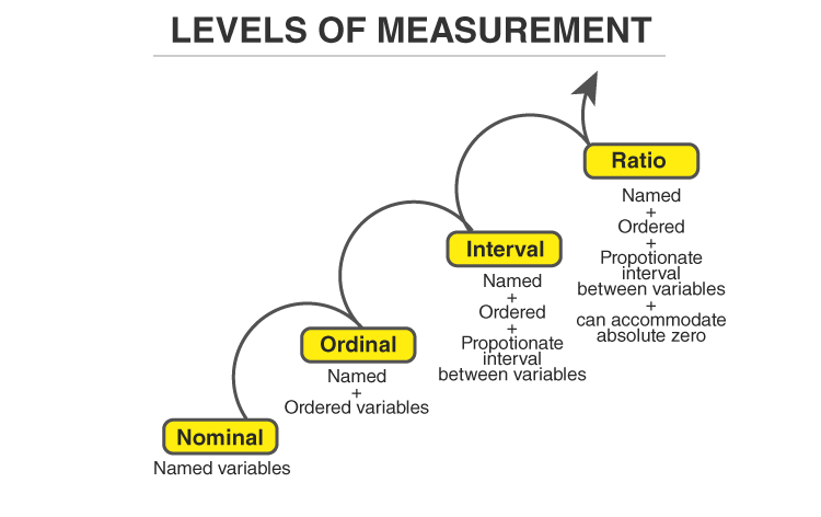
Nominal Scale

A nominal scale is the 1st level of measurement scale in which the numbers serve as “tags” or “labels” to classify or identify the objects. A nominal scale usually deals with the non-numeric variables or the numbers that do not have any value.

Characteristics of Nominal Scale

• A nominal scale variable is classified into two or more categories. In this measurement mechanism, the answer should fall into either of the classes.
• It is qualitative. The numbers are used here to identify the objects.
• The numbers don’t define the object characteristics. The only permissible aspect of numbers in the nominal scale is “counting.”

Example:

An example of a nominal scale measurement is given below:

What is your gender?

M- Male

F- Female

Here, the variables are used as tags, and the answer to this question should be either M or F.

Ordinal Scale

The ordinal scale is the 2nd level of measurement that reports the ordering and ranking of data without establishing the degree of variation between them. Ordinal represents the “order.” Ordinal data is known as qualitative data or categorical data. It can be grouped, named and also ranked.

Characteristics of the Ordinal Scale

• The ordinal scale shows the relative ranking of the variables
• It identifies and describes the magnitude of a variable
• Along with the information provided by the nominal scale, ordinal scales give the rankings of those variables
• The interval properties are not known
• The surveyors can quickly analyse the degree of agreement concerning the identified order of variables

Example:

• Ranking of school students – 1st, 2nd, 3rd, etc.
• Ratings in restaurants
• Evaluating the frequency of occurrences
  • Very often
  • Often
  • Not often
  • Not at all
• Assessing the degree of agreement
  • Totally agree
  • Agree
  • Neutral
  • Disagree
  • Totally disagree

Interval Scale

The interval scale is the 3rd level of measurement scale. It is defined as a quantitative measurement scale in which the difference between the two variables is meaningful. In other words, the variables are measured in an exact manner, not as in a relative way in which the presence of zero is arbitrary.

Characteristics of Interval Scale:

• The interval scale is quantitative as it can quantify the difference between the values
• It allows calculating the mean and median of the variables
• To understand the difference between the variables, you can subtract the values between the variables
• The interval scale is the preferred scale in Statistics as it helps to assign any numerical values to arbitrary assessment such as feelings, calendar types, etc.

Example:

• Likert Scale
• Net Promoter Score (NPS)
• Bipolar Matrix Table

Ratio Scale

The ratio scale is the 4th level of measurement scale, which is quantitative. It is a type of variable measurement scale. It allows researchers to compare the differences or intervals. The ratio scale has a unique feature. It possesses the character of the origin or zero points.

Characteristics of Ratio Scale:

• Ratio scale has a feature of absolute zero
• It doesn’t have negative numbers, because of its zero-point feature
• It affords unique opportunities for statistical analysis. The variables can be orderly added, subtracted, multiplied, divided. Mean, median, and mode can be calculated using the ratio scale.
• Ratio scale has unique and useful properties. One such feature is that it allows unit conversions like kilogram – calories, gram – calories, etc.

Example:

An example of a ratio scale is:

What is your weight in Kgs?

• Less than 55 kgs
• 55 – 75 kgs
• 76 – 85 kgs
• 86 – 95 kgs
• More than 95 kgs

For more information related to Statistics-concepts, register at BYJU’S – The Learning App and also learn relevant Mathematical concepts.